Visual Python

[agor95]

I have been looking around for a general Visual Programing product.

https://en.wikipedia.org/wiki/VPython

This is the one I am looking at anyone that is interested in supplying Bessler related demos.

Here is the place.

[Furcurequs]

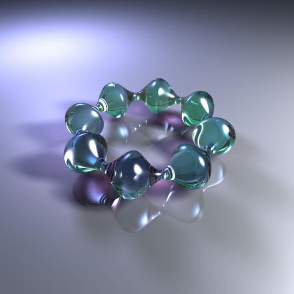
I used a python script and the free (for non-commercial use) python module of the Lightflow Rendering Tools to generate this image many years ago now:



I did use a modeling program to generate the cup geometry, but I wrote my own python module to import that geometry into my scene. The table and sphere I simply scripted in python itself. (ETA: After reading what I said in another thread and rethinking things, I believe I could have imported the geometry for the sphere instead of scripting it, but scripting it would have been simple enough.)

Here is an image of one of the examples that came with the Lightflow module. It was entirely scripted and so the object was generated with a math equation rather than a 3D modeler.



http://www.lightflowtech.com/images/bspline5_b.jpg

I've also scripted and rendered (the frames for) some simple animations, but of course with the python language it should also be possible to do proper mathematical modeling and thus generate a decent simulation.

You would have to use an older version of Python with these rendering tools, however.

Lightflow Rendering Tools
Python Module 1.5

The Python Module is an extension for the Python language incorporating almost all of the Lightflow Rendering Tools.

This tool is meant for advanced 3d users who don't need any 3d modeling tool to develop their own scenes, and still prefer simple scripting...

Supported platforms include Linux and Windows NT.

This trial product is completely free for non commercial uses.

http://www.lightflowtech.com/news.html

http://www.lightflowtech.com

I've also done some simple animations with the scripted ray tracer POV-Ray. It's own built in scripting language is probably powerful enough to do what we would need to do, too. It seemed to be quite similar to that used with the Python Lightflow module.

http://www.povray.org/

Dwayne

ETA: I've also found this - someone who has written a Python library called Vapory so that POV-Ray can be used directly from Python itself:

Things You Can Do With Python and POV-Ray

This post presents Vapory, a library I wrote to bring POV-Ray’s 3D rendering capabilities to Python.

http://zulko.github.io/blog/2014/11/13/ ... d-pov-ray/

ETA2: Here's one of the frames of something I scripted and rendered with POV-Ray (without using any sort of Python library). It's not meant to be any sort of Bessler wheel design, btw.



Here's the link to the small animation:

http://www.besslerwheel.com/forum/files/flywheel.mpg

Here's the link to the original thread:

http://www.besslerwheel.com/forum/viewt ... p?p=107011

Here's the thread in which I first posted the above Lightflow image:

"Golems 3d sandbox physics simulation program"

http://www.besslerwheel.com/forum/viewt ... p?p=137284

I rendered the frames for this animation using Python and the Lightflow Rendering Tools Python module. I think it is close to 3 MB in size. It's a shame Lightflow cannot be used for commercial use.

http://www.besslerwheel.com/forum/files/dvd.mpg

[agor95]

I think Blender also can be used by python scripts.

It is all about using the right tool for the job; that the right time.

[agor95]

I have been working on the V Python scripts.

So far it's been a process of dynamic illustration development.
Instead of POV [blender like] static images.

Also I have been getting my head around formula graphing in the same product.

That will lead to demo simulation with graphical support documentation.

P.S. The product is not restricted to XY simulations.

The Unicode of formula is done and has been implemented on two private web servers.

[agor95]

Here is the script and graphs that appear when run in Visual Python.

Code: Select all

from __future__ import print_function, division
from visual.graph import *

print("""
Formula Horizontal Rorationg System
""")

# Using a graph-plotting module

t = 0

mass = 1            # [kg]
r    = 2            # [m]         Radius
v    = 1            # [m/s]       velocity

Rinc = -0.1         # [m]   Reduction in Radius

ltv  = 1            # [m/s] Linear Tangental Velocity
wi   = 0            # [j]   Work Increment
wt   = 0            # [j]   Work Total

#ltv = ((t*Rinc)+r) * v / (((t+1)*Rinc)+r)
ke = 0.5*mass*v**2                                       # [j] Kinetic Energy         'KE'
cf = mass*((ltv+v)/2)**2/((((t+1)*Rinc+r)+(t*Rinc+r))/2) # [N] Centripital Force      'CF'
am = r*mass*v                                            # [kg m2/s] Angular Momentun 'L'
lm = mass*v                                              # [kg m/s] Linear Momentum   'p'

# Rotational Check of energy

moi = mass*r**2     # [kg m2]     Moment of Inertia
av = ltv/r          # [radians/s] Angular Volocity
rke = 0.5*moi*av**2 # [j]         Rotational Kinetic Energy

# If xmax, xmin, ymax, or ymin specified, the related axis is not autoscaled
# Can turn off autoscaling with
#    linera.autoscale[0]=0 for x or oscillation.autoscale[1]=0 for y

linera = gdisplay(x=0,y=0,title='Horizontal Rotating System',xtitle='Count', ytitle='Response (click and drag mouse to see coordinates)')
funct1 = gcurve(display=linera,color=color.cyan)
funct2 = gcurve(display=linera,color=color.red)
funct3 = gcurve(display=linera,color=color.yellow)
funct4 = gcurve(display=linera,color=color.blue)
funct5 = gcurve(display=linera,color=color.green)

Rotate = gdisplay(x=0,y=400,title='Rotational check of Energy',xtitle='Count', ytitle='Response (click and drag mouse to see coordinates)')
funct6 = gcurve(display=linera,color=color.cyan)
funct7 = gcurve(display=linera,color=color.red)
funct8 = gcurve(display=linera,color=color.yellow)

#funct2 = gvbars(delta=0.5, color=color.red)
#funct3 = gdots(color=color.yellow)

for t in arange(0, 11, 1):

    # ltv cyan
#    print (ltv)
    funct1.plot( pos=(t,ltv))
    ltv = ((t*Rinc+r) * v) /((t+1)*Rinc+r)

    # ke red
    ke = 0.5*mass*v**2
#    print (ke)
    funct2.plot( pos=(t,ke))
    
    # cf yellow
#    print (cf)
    funct3.plot( pos=(t,cf))
    cf = mass*((ltv+v)/2)**2/((((t+1)*Rinc+r)+(t*Rinc+r))/2)
    
    # am blue
##    print (am)
##    funct4.plot( pos=(t,am))
    
    # lm blue

    lm = mass*v

#    print (lm)
    funct5.plot( pos=(t,lm))

    
    # moi green
    
    moi = mass*(t*Rinc+r)**2

#    print (moi)
    funct6.plot( pos=(t,moi))

    # W angular velocity
    
    av = v / (t*Rinc+r)

#    print (av)
    funct7.plot( pos=(t,av))
    
    # ke rotational kinetic energy
    
    rke =  0.5*moi*av**2

#    print (rke)
    funct8.plot( pos=(t,rke))

    v = ltv

[ME]

Interesting, and nice to see an example.

It appears you calculate the wrong value for several graphs: you first plot and then calculate *) - it makes a difference because (I guess) your step-size is 10% of the range. A bit strange it doesn't include t=11.
Perhaps it's an idea to do the calculations first in a single block of code, and then plot in a second block of code; so you can separate calculus and output.

Do you need to do all the physics calculations yourself, or does it also include a library?

*) ok, I noticed (t+1)

[agor95]

I used an excel example supplied in another topic.

Then cut down one of the Visual Python examples; that contained graphs.

Next

I used the print lines (they are now commented out #).

Did what was required to get the same results as the excel.

commented the prints and entered the pot commands.

for t in arange(0, 11, 1): gives t counting from 0 to 10

Python is really powerfully - it's motto is 'batteries included'

There is a world of Python solutions out there. Nasa & Google etc.

This is a simple and relevant example.

I recommend down loading the free V Python and run the doublependulum script example.

[ME]

Installed it.
It looks like you still need to handle all physics (especially collisions) yourself.
Although the basic physics can be captured in formulas, some combinations need to be solved in a numerical way.
That's a lot of work before getting good results.

[agor95]

You will see the 'from visual.graph import *'

This is a library of commands for 3d visualization.
There are other libraries for doing other things.

I look forward to a day we can type

'from bessler import wheel *'

regards

[agor95]

This script creates two graphs showing force [Newtons] using a
4lb weight; Red is Gravity and the yellow is CF.

There are two rotation rates 26rpm and 20rpm.

Code: Select all

from __future__ import print_function, division
from visual.graph import *

print("""
Formula Acceleration dur to Rotation [AR] vs Acceleration due to Gravity [AG]
""")

# Using a graph-plotting module

# If xmax, xmin, ymax, or ymin specified, the related axis is not autoscaled
# Can turn off autoscaling with
#    linera.autoscale[0]=0 for x or oscillation.autoscale[1]=0 for y

Rotate = gdisplay(x=0,y=0,title='26 RPM Radious 12 feet Rotating System',xtitle='Radious', ytitle='Response (click and drag mouse to see coordinates)')
funct1 = gcurve(display=Rotate,color=color.red)
funct3 = gcurve(display=Rotate,color=color.yellow)

Rotate2 = gdisplay(x=0,y=400,title='20 RPM Radious 12 feet Rotating System',xtitle='Radious', ytitle='Response (click and drag mouse to see coordinates)')
funct6 = gcurve(display=Rotate2,color=color.red)
funct8 = gcurve(display=Rotate2,color=color.yellow)

#
# initial values
#

g = 9.81

mass  = 1.81437    # 4lb in [kg]

dr = 0.1           # delta radious
r     = 0          # [m] Radius

#
# initial calculations
#

# Rotational Check of energy

av = (2.0*(22.0/7.0))/(60.0/26.0)       # [radians/s] Angular Volocity RPM 26

av2 = (2.0*(22.0/7.0))/(60.0/20.0)      # [radians/s] Angular Volocity RPM 20

cf = mass*0*av**2

cf2 = mass*0*av2**2

moi = mass*1.8288**2                    # [kg m^2]    Moment of Inertia
rke = 0.5*moi*av**2                     # [j] Rotational Kinetic Energy

print (rke)

#
# recalculate loop
#

for r in arange(0.0, 1.8288+dr, dr):

    # g red
#    print (g)
    funct1.plot( pos=(r,g*mass))
    funct6.plot( pos=(r,g*mass))
    
    # cf yellow
#    print (cf)

    cf = mass*r*av**2

    funct3.plot( pos=(r,cf))

    cf2 = mass*r*av2**2

    funct8.plot( pos=(r,cf2))

[agor95]

If you follow bessler's cues then you may get to this idea.
Allow a weight on the hub drop for 135 degrees clockwise.
bounce the weight off the hub and collect it again.
This is test 1 were the weight/ball is separated from the hub.
However with the hub rotating at the correct rate you can
get the effect.

So the weight drops 9 feet and only need to be lifted around 4 feet.

Code: Select all

from __future__ import division
from visual import *

print("""
Right button drag to rotate "camera" to view scene.
  On a one-button mouse, right is Command + mouse.
Middle button to drag up or down to zoom in or out.
  On a two-button mouse, middle is left + right.
  On a one-button mouse, middle is Option + mouse.

This example one shows a bouncing ball next to a rotating hub.


""")

Myscene = display(title='Rotator',
                  x=0,y=0,width=800, height=800,
                  center=(0,0,0), background=(0,0,0),foreground=(1,1,1),
                  ambient=color.gray(0.2),
                  lights=
                  [distant_light(direction=(0.22, 0.44, 0.88), color=color.gray(0.8)),
                   distant_light(direction=(-0.88, -0.22, -0.44), color=color.gray(0.3))])


Myscene.cursor.visible = True    #Default

# How fast the render process takes in milliseconds
Myscene.show_rendertime = False

# Default close the screen closes the program
Myscene.exit = True

dpth  = 0.5
lth = 6

# Center of the hub
point  = sphere(radius=dpth, color=color.yellow)

# rotate the whole hub
frame0 = frame(pos=(0,0,0), axis=(0,1,0))

# The spokes
theta1 = 0
frame1 = frame(frame=frame0, pos=(0,0,0), axis=(0,0,1))
box1 = box(frame=frame1, y=lth/2+1*dpth, size=(dpth,5,dpth))
frame1.rotate(axis=(0,0,1), angle=theta1)

theta2 = -0.25*pi
frame2 = frame(frame=frame0, pos=(0,0,0), axis=(0,0,1))
box2 = box(frame=frame2, y=lth/2+1*dpth, size=(dpth,5,dpth))
frame2.rotate(axis=(0,0,1), angle=theta2)

theta3 = -0.5*pi
frame3 = frame(frame=frame0, pos=(0,0,0), axis=(0,0,1))
box3 = box(frame=frame3, y=lth/2+1*dpth, size=(dpth,5,dpth), color=color.red)
frame3.rotate(axis=(0,0,1), angle=theta3)

theta4 = -0.75*pi
frame4 = frame(frame=frame0, pos=(0,0,0), axis=(0,0,1))
box4 = box(frame=frame4, y=lth/2+1*dpth, size=(dpth,5,dpth))
frame4.rotate(axis=(0,0,1), angle=theta4)

theta5 = -1*pi
frame5 = frame(frame=frame0, pos=(0,0,0), axis=(0,0,1))
box5 = box(frame=frame5, y=lth/2+1*dpth, size=(dpth,5,dpth))
frame5.rotate(axis=(0,0,1), angle=theta5)

theta6 = -1.25*pi
frame6 = frame(frame=frame0, pos=(0,0,0), axis=(0,0,1))
box6 = box(frame=frame6, y=lth/2+1*dpth, size=(dpth,5,dpth))
frame6.rotate(axis=(0,0,1), angle=theta6)

theta7 = -1.5*pi
frame7 = frame(frame=frame0, pos=(0,0,0), axis=(0,0,1))
box7 = box(frame=frame7, y=lth/2+1*dpth, size=(dpth,5,dpth))
frame7.rotate(axis=(0,0,1), angle=theta7)

theta8 = -1.75*pi
frame8 = frame(frame=frame0, pos=(0,0,0), axis=(0,0,1))
box8 = box(frame=frame8, y=lth/2+1*dpth, size=(dpth,5,dpth))
frame8.rotate(axis=(0,0,1), angle=theta8)

# The base block
floor1 = box(pos=(0,-5.5,-1), length=16, height=0.5, width=1, color=color.blue)
floor2 = box(pos=(-7.5,-5.5,0), length=1, height=0.5, width=1, color=color.blue)
floor3 = box(pos=(7.5,-5.5,0), length=1, height=0.5, width=1, color=color.blue)
floor4 = box(pos=(0,-5.5,1), length=16, height=0.5, width=1, color=color.blue)

frame9 = frame(pos=(4.5,-5.5,1), axis=(0,0,1))
bouncpaddle1 = box(frame=frame9, length=1, height=0.5, width=1.5, color=color.yellow)
frame9.rotate(axis=(0,0,1), angle=pi/4)

ball = sphere(pos=(4,6-0.25,1), radius=0.5, color=color.green,opacity=0.5)
ball.velocity = vector(0,-1,0)

dt = 0.005
t = 0.

dtheta1 = 0.

while t < 2&#58;
    rate&#40;50&#41; # 50 loop per second

    frame0.rotate&#40;axis=&#40;0,0,1&#41;, angle=-dtheta1&#41;
    dtheta1 = 1.75*dt

    ball.pos = ball.pos + ball.velocity*dt

    if ball.y < -5.5+0.75&#58;
        ball.velocity.y = -ball.velocity.y
        ball.velocity.x = -ball.velocity.y
    else&#58;
        ball.velocity.y = ball.velocity.y - 9.8*dt
        if ball.x > 4&#58;
            ball.velocity.x = 0

    if ball.x < -6+0.25&#58;
         ball.velocity.x = -ball.velocity.x
 

    t = t+dt

[agor95]

Simple 1 second bounce ten times.

I wanted to get the timing aspect up to speed.

Copy te code into a text files and load it in V python.
previously installed

You can comment out this section:

Code: Select all

from __future__ import division
from visual import *
from visual.graph import *

import time

Myscene = display(title='Ten Second Bounce',
                  x=0,y=0,width=800, height=400,
                  center=(0,0,0), background=(0,0,0),foreground=(1,1,1),
                  ambient=color.gray(0.2),
                  lights=
                  [distant_light(direction=(0.22, 0.44, 0.88), color=color.gray(0.8)),
                   distant_light(direction=(-0.88, -0.22, -0.44), color=color.gray(0.3))])

vhight = gdisplay(x=1, y=400, xtitle='Time', ytitle='Response (click and drag mouse to see coordinates)')
funct1 = gcurve(color=color.cyan)
#funct2 = gvbars(delta=0.5, color=color.red)
#funct3 = gdots(color=color.yellow)


#Myscene.background=(1,1,1)
#Myscene.foreground=(0,0,0)
#Myscene.ambient=color.gray(0.2)

Myscene.cursor.visible = True    #Default

# How fast the render process takes in milliseconds
Myscene.show_rendertime = True

Myscene.select()

# Default close the screen closes the program
Myscene.exit = True

# controlling the view
#Myscene.autocenter = True

# range or scale
# scale (0.1,0.1,0.1) same as range (10.10.10)
Myscene.autoscale = True        #Default
# Myscene.scale = 1

#
# Mouse Interactions
#
def pause():
    while True:
        rate(50)
        if Myscene.mouse.events:
            m = Myscene.mouse.getevent()
            if m.click == 'left': return
        elif Myscene.kb.keys:
            k = Myscene.kb.getkey()
            return

#
# clock
#
def hourminute():
    now = time.localtime(time.time())
    hour = now[3] % 12
    minute = now[4]
    second = now[5]
    return (hour, minute,second)

class analog_clock:
    def __init__(self, pos=(0,0,0), radius=1., axis=(0,0,1)):
        self.pos = vector(pos)
        self.axis = vector(axis)
        self.radius = radius
        self.spheres = []
        self.hour = 0
        self.minute = -1
        for n in range(12):
            self.spheres.append(sphere(pos=self.pos+rotate(radius*scene.up,
                    axis=self.axis, angle=-2.*pi*n/12.), radius=radius/20.,
                    color=color.hsv_to_rgb((n/12.,1,1)) ))
        self.hand = arrow(pos=pos, axis=0.95*radius*scene.up,
                    shaftwidth=radius/10., color=color.cyan)
        self.update()
        
    def update(self):
        hour, minute, second = hourminute()
        if self.hour == hour and self.minute == minute: return
        self.hand.axis = rotate(0.95*self.radius*scene.up,
                    axis=self.axis, angle=-2.*pi*minute/60.)
        self.spheres[self.hour].radius = self.radius/20.
        self.spheres[hour].radius = self.radius/10.
        self.hour = hour
        self.minute = minute
        self.second = second

# Decorate back slab with a gold box and a clock
##box(pos=(0,h/2.,-R+d/2+0.1), size=(w/2.,w/2.,0.2), 
##    color=(1,0.8,0), material=materials.wood)
##clock = analog_clock(pos=(0,h/2.,-R+d/2+0.2+0.2*h/10),
##                    radius=0.2*w, axis=(0,0,1))

    # Update the analog clock on the back slab
##    clock.update()

print('Pausing')

#pause()

#point = sphere(pos=(0.,0.25,1.), radius=0.5,color=color.yellow)

# top surface of floor y = 0
floor = box(pos=(0.,-0.5,0.),length=8, height=0.5, width=8, color=color.blue)

# bottom of ball - not it's centor
ball = sphere(pos=(0.,(9.81/8)+0.25,0.), radius=0.5, color=color.red)
ball.velocity = vector(0.,0.,0.)
ball.mass = 1.81437 # 4lb in kg

dt = 0.001
t  = 0.

hour, minute, second = hourminute()

s = str(hour)+":"+str(minute)+":"+str(second)
print(s)

while t < 10&#58;
    rate&#40;1/dt&#41;
    ball.pos = ball.pos + ball.velocity*dt
    if ball.y < 0.25&#58;
        ball.velocity.y = -ball.velocity.y
    else&#58;
        ball.velocity.y = ball.velocity.y - 9.81*dt

    funct1.plot&#40;pos=&#40;t,ball.y-0.25&#41;&#41;

    t = t + dt
#    pause&#40;&#41;

hour, minute, second = hourminute&#40;&#41;

s = str&#40;hour&#41;+"&#58;"+str&#40;minute&#41;+"&#58;"+str&#40;second&#41;
print&#40;s&#41;

[agor95]

For those with up to date browsers

http://doc.x3dom.org/tutorials/animatio ... ample.html

If you see a house you can walk around it.

This proves you would be able to see a moving Bessler illustrations in 3D using your browser.

[agor95]

Just a test for new browser users

http://steampunk.ddns.net/cube.html

[agor95]

http://steampunk.ddns.net/face.html